Chapter 7 dplyr and Pivot Tables
7.1 Summary
Pivot tables are powerful tools in Excel for summarizing data in different ways. We will create these tables using the group_by and summarize functions from the dplyr package (part of the Tidyverse). We will also learn how to format tables and practice creating a reproducible report using RMarkdown and sharing it with GitHub.
7.2 Objectives
In R, we can use dplyr for pivot tables by using 2 main verbs in combination: group_by and summarize. We will also continue to emphasize reproducibility in all our analyses.
- Discuss pivot tables in Excel
- Introduce
group_by() %>% summarize()from thedplyrpackage - Practice our reproducible workflow with RMarkdown and GitHub
7.3 Resources
- dplyr.tidyverse.org
- R for Data Science: Transform Chapter
- Intro to Pivot Tables I-III by Excel Campus (YouTube)
7.4 Pivot table overview
Wikipedia describes a pivot table as a “table of statistics that summarizes the data of a more extensive table…This summary might include sums, averages, or other statistics, which the pivot table groups together in a meaningful way.” Fun fact: it also says that “Although pivot table is a generic term, Microsoft trademarked PivotTable in the United States in 1994.”
Pivot tables are a really powerful tool for summarizing data, and we can have similar functionality in R — as well as nicely automating and reporting these tables. We will learn about this using data about lobsters and will go back and forth between R and Excel as we learn.
Let’s start off in R, and have a look at the data.
7.5 RMarkdown setup
Let’s start a new RMarkdown file in our repo, at the top-level (where it will be created by default in our Project). I’ll call mine pivot_lobsters.Rmd.
In the setup chunk, let’s attach our libraries and read in our lobster data. In addition to the tidyverse package we will also use the skimr package. You will have to install it, but don’t want it to be installed every time you write your code. The following is a nice convention for having the install instructions available (on the same line) as the library() call.
## attach libraries
library(tidyverse)
library(readxl)
library(here)
library(skimr) # install.packages('skimr')

## read in data
lobsters <- read_xlsx(here("data/lobsters.xlsx"))
Let’s add a code chunk and explore the data in a few ways.
## # A tibble: 6 x 7
##    year month date    site  transect replicate size_mm
##   <dbl> <dbl> <chr>   <chr>    <dbl> <chr>       <dbl>
## 1  2012     8 8/20/12 ivee         3 A              70
## 2  2012     8 8/20/12 ivee         3 B              60
## 3  2012     8 8/20/12 ivee         3 B              65
## 4  2012     8 8/20/12 ivee         3 B              70
## 5  2012     8 8/20/12 ivee         3 B              85
## 6  2012     8 8/20/12 ivee         3 C              60
head() gives us a look at the first rows of the data (6 by default). I like this because I can see the column names and get a sense of the shape of the data. I can also see the class of each column (double or character)
In this data set, every row is a unique observation. This is called “uncounted” data; you’ll see there is no row for how many lobsters were seen because each row is an observation, or an “n of 1”.
##       year          month           date               site
##  Min.   :2012   Min.   :8.000   Length:6366        Length:6366
##  1st Qu.:2015   1st Qu.:8.000   Class :character   Class :character
##  Median :2017   Median :8.000   Mode  :character   Mode  :character
##  Mean   :2016   Mean   :8.017
##  3rd Qu.:2018   3rd Qu.:8.000
##  Max.   :2018   Max.   :9.000
##
##     transect      replicate            size_mm
##  Min.   :1.000   Length:6366        Min.   : 18.00
##  1st Qu.:2.000   Class :character   1st Qu.: 65.00
##  Median :4.000   Mode  :character   Median : 75.00
##  Mean   :3.806                      Mean   : 73.02
##  3rd Qu.:5.000                      3rd Qu.: 82.00
##  Max.   :9.000                      Max.   :183.00
##                                     NA's   :6
summary gives us summary statistics for each variable (column). I like this for numeric columns, but it doesn’t give a lot of useful information for non-numeric data. To have a look there I like using the skimr package:
| Name | lobsters |
| Number of rows | 6366 |
| Number of columns | 7 |
| _______________________ | |
| Column type frequency: | |
| character | 3 |
| numeric | 4 |
| ________________________ | |
| Group variables | None |
Variable type: character
| skim_variable | n_missing | complete_rate | min | max | empty | n_unique | whitespace |
|---|---|---|---|---|---|---|---|
| date | 0 | 1 | 6 | 7 | 0 | 38 | 0 |
| site | 0 | 1 | 4 | 4 | 0 | 5 | 0 |
| replicate | 0 | 1 | 1 | 1 | 0 | 4 | 0 |
Variable type: numeric
| skim_variable | n_missing | complete_rate | mean | sd | p0 | p25 | p50 | p75 | p100 | hist |
|---|---|---|---|---|---|---|---|---|---|---|
| year | 0 | 1 | 2016.24 | 1.66 | 2012 | 2015 | 2017 | 2018 | 2018 | ▁▁▂▂▇ |
| month | 0 | 1 | 8.02 | 0.13 | 8 | 8 | 8 | 8 | 9 | ▇▁▁▁▁ |
| transect | 0 | 1 | 3.81 | 2.17 | 1 | 2 | 4 | 5 | 9 | ▇▆▅▃▂ |
| size_mm | 6 | 1 | 73.02 | 13.61 | 18 | 65 | 75 | 82 | 183 | ▁▇▂▁▁ |
This skimr:: notation is a reminder to me that skim is from the skimr package. It is a nice convention: it’s a reminder to others (especially you!).
skim lets us look more at each variable. I particularly like looking at missing data. There are 6 missing values in the size_mm variable.
We can also make a quick plot to have a look at these data, and use our new ggplot2 skills. Let’s make a bar chart by year for each site
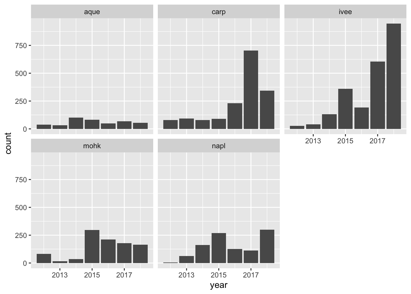
(geom_bar() counts things and geom_col() is for values within the data (mean))
7.5.1 Our task
So this is all great to get a quick look. But what if we needed to report to someone about how the average size of lobsters has changed over time across sites?
To answer this we need to do a pivot table in Excel, or data wrangling in R.
Let’s start by having a quick look at what pivot tables can do in Excel.
7.6 Pivot table demo
Let’s make a pivot table with our lobster data.
Let’s start off with how many lobsters were counted each year. I want a count of rows by year.
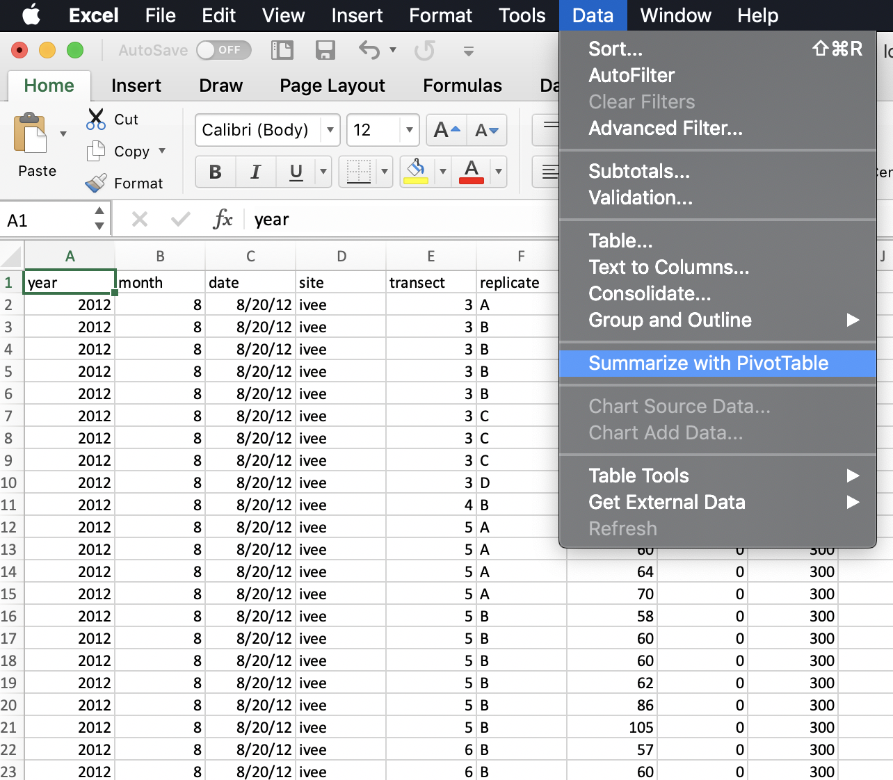
So to do this in Excel we would initiate the Pivot Table Process:
And it will do its best to find the data I would like to include in my Pivot Table (it can have difficulty with non-rectangular or “non-tidy” data), and suggest we make this in a new sheet:
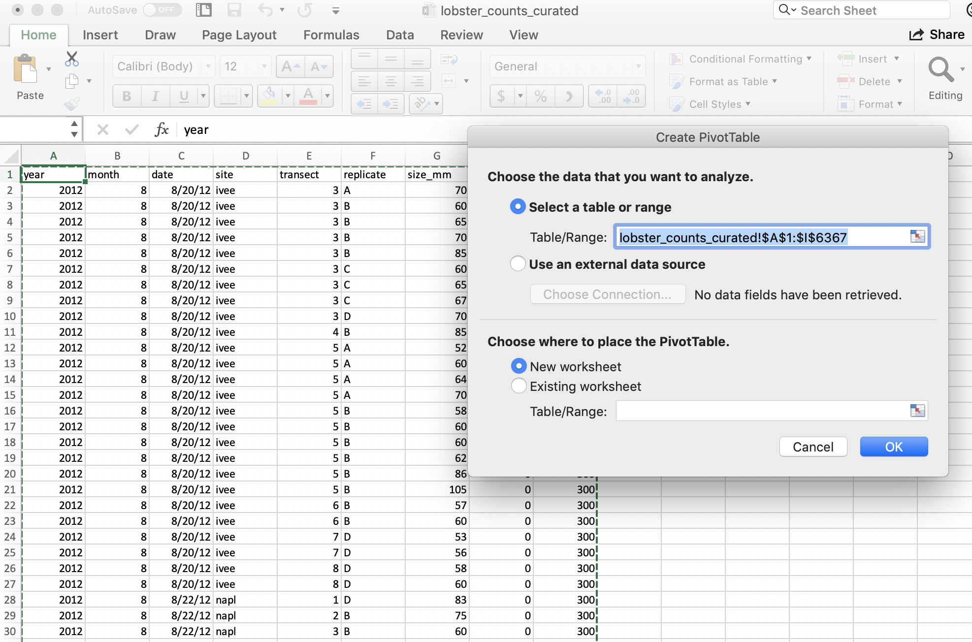
And then we’ll get a little wizard to help us create the Pivot Table.
7.6.1 pivot one variable
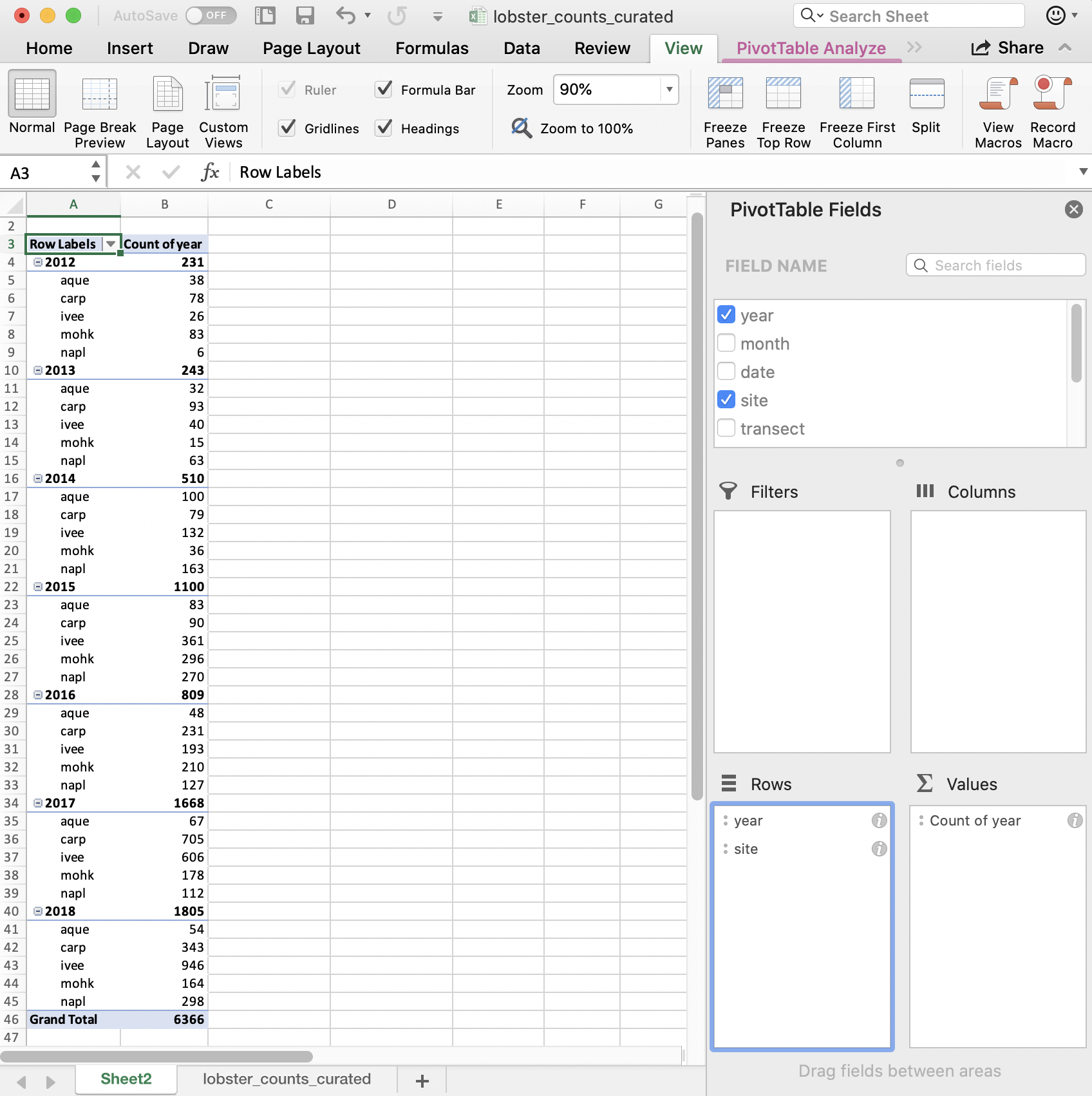
I want to summarize by year, so I drag “year” down into the “Rows” box, and to get the counts by year I actually drag the same variable, “year” into the “Values” box. And it will create a Pivot Table for me! But “sum” as the default summary statistic, so I can click the little “I” icon to change this to count.
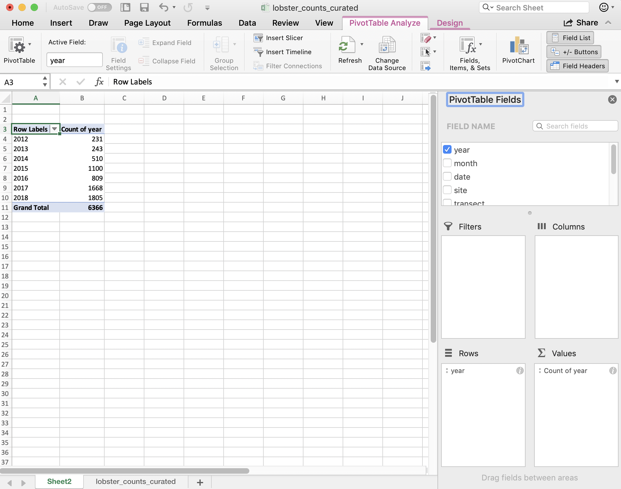
A few things to note:
- The pivot table is separate entity from our data (it’s on a different sheet); the original data has not been affected
- The pivot table only shows the variables we requested; we don’t see other columns (like date, month, or site).
- Notice that in Excel we retain the overall totals for each site (in bold, on the same line with the site name). This is nice for communicating about data. But it can be problematic for further analyses, because it could be easy to take a total of this column and introduce errors.
So pivot tables are great because they summarize the data and keep the raw data raw — they even promote good pratice because they by default ask you if you’d like to present the data in a new sheet rather than in the same sheet.
7.6.2 pivot two variables
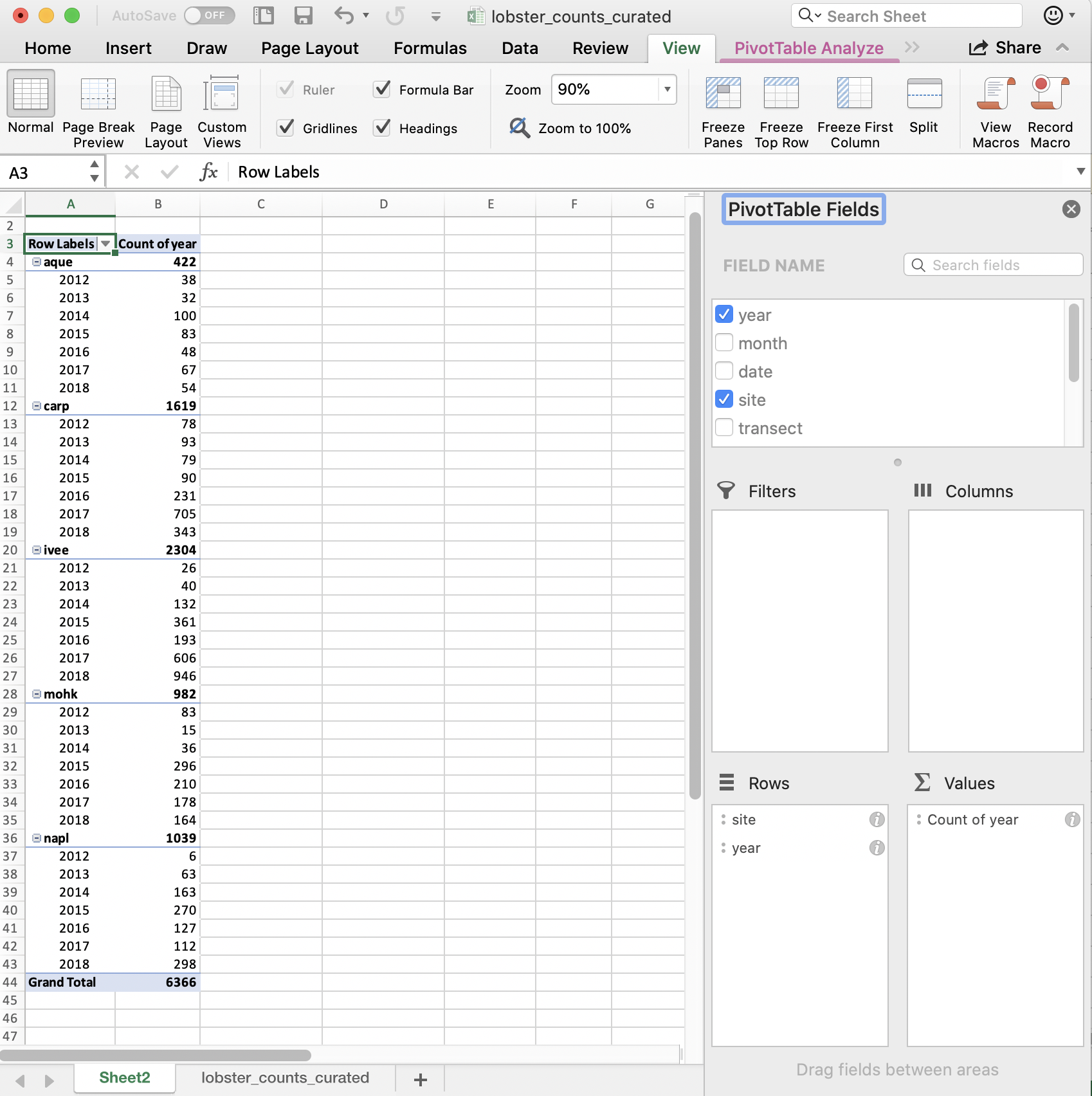
We can also add site as a second variable by dragging it:
And then can reverse the order by dragging:
So in terms of our final interest of average size by site and year, we are on our way! I’m going to stop here because we want to be able to do this in R.
The power of R is in the automation, and in keeping that raw data truly raw.
Let’s talk about how this looks like in R.
7.7 group_by() %>% summarize()
In R, we can create the functionality of pivot tables by using 2 main dplyr verbs in combination: group_by and summarize.
Say it with me: “pivot tables are group_by and then summarize”. And just like pivot tables, you have flexibility with how you are going to summarize. For example, we can calculate an average, or a total.
I think it’s incredibly powerful to visualize what we are talking about with our data when do do these kinds of operations. It looks like this (from RStudio’s cheatsheet; all cheatsheets available from https://rstudio.com/resources/cheatsheets):
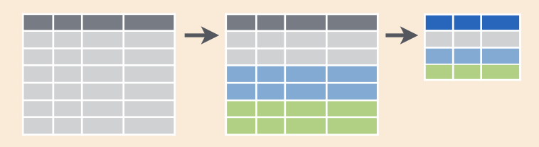
When we were reporting by year or site, we were essentially modifying what we were grouping by (the different colors here in this figure.
Let’s do this in R.
7.7.1 group_by one variable
Let’s try this on our lobsters data, just like we did in Excel. We will count the the total number of lobster by year. In R vocabulary, we will group_by year and then summarize by counting using n(), which is a function from dplyr. n() counts the number of times an observation shows up, and since this is uncounted data, this will count each row. We’ll also use the pipe operator %>%, which you can read as “and then”.
This to me reads: “take the lobsters data and then group_by year and then summarize by count in a new column called ‘count’”
## # A tibble: 7 x 2
##    year count_by_year
##   <dbl>         <int>
## 1  2012           231
## 2  2013           243
## 3  2014           510
## 4  2015          1100
## 5  2016           809
## 6  2017          1668
## 7  2018          1805
Notice how together, group_by and summarize minimize the amount of information we see. We also saw this with the pivot table. We lose the other columns that aren’t involved here.
Question: What if you don’t group_by first? Let’s try it and discuss what’s going on.
## # A tibble: 1 x 1
##   count
##   <int>
## 1  6366
So if we don’t group_by first, we will get a single summary statistic (sum in this case) for the whole dataset.
Another question: what if we only group_by?
## # A tibble: 6,366 x 7
## # Groups:   year [7]
##     year month date    site  transect replicate size_mm
##    <dbl> <dbl> <chr>   <chr>    <dbl> <chr>       <dbl>
##  1  2012     8 8/20/12 ivee         3 A              70
##  2  2012     8 8/20/12 ivee         3 B              60
##  3  2012     8 8/20/12 ivee         3 B              65
##  4  2012     8 8/20/12 ivee         3 B              70
##  5  2012     8 8/20/12 ivee         3 B              85
##  6  2012     8 8/20/12 ivee         3 C              60
##  7  2012     8 8/20/12 ivee         3 C              65
##  8  2012     8 8/20/12 ivee         3 C              67
##  9  2012     8 8/20/12 ivee         3 D              70
## 10  2012     8 8/20/12 ivee         4 B              85
## # … with 6,356 more rows
7.7.2 RStudio Viewer
Let’s now check the lobsters variable. We can do this by clicking on lobsters in the Environment pane in RStudio.
We see that we haven’t changed any of our original data that was stored in this variable. (Just like how the pivot table didn’t affect the raw data on the original sheet).
Aside: You’ll also see that when you click on the variable name in the Environment pane,
View(lobsters)shows up in your Console.View()(capital V) is the R function to view any variable in the viewer. So this is something that you can write in your RMarkdown script, although RMarkdown will not be able to knit this view feature into the formatted document. So, if you want includeView()in your RMarkdown document you will need to either comment it out#View()or addeval=FALSEto the top of the code chunk so that the full line reads{r, eval=FALSE}.
7.7.3 group_by multiple variables
Great. Now let’s summarize by both year and site like we did in the pivot table. We are able to group_by more than one variable. Let’s do this together:
## # A tibble: 35 x 3
## # Groups:   site [5]
##    site   year count_by_siteyear
##    <chr> <dbl>             <int>
##  1 aque   2012                38
##  2 aque   2013                32
##  3 aque   2014               100
##  4 aque   2015                83
##  5 aque   2016                48
##  6 aque   2017                67
##  7 aque   2018                54
##  8 carp   2012                78
##  9 carp   2013                93
## 10 carp   2014                79
## # … with 25 more rows
text.
7.7.4 summarize multiple variables
We can summarize multiple variables at a time. So far we’ve done the count of lobster observations. Let’s also do the mean and standard deviation. First let’s use the mean() function to calculate the mean. We do this within the same summarize() function, but we can add a new line to make it easier to read. Notice how when you put your curser within the parenthesis and hit return, the indentation will automatically align.
lobsters %>%
  group_by(site, year) %>%
  summarize(count_by_siteyear =  n(),
            mean_size_mm = mean(size_mm))
## # A tibble: 35 x 4
## # Groups: site [5]
## site year count_by_siteyear mean_size_mm
## <chr> <dbl> <int> <dbl>
## 1 aque 2012 38 71
## 2 aque 2013 32 72.1
## 3 aque 2014 100 76.9
## 4 aque 2015 83 68.5
## 5 aque 2016 48 68.7
## 6 aque 2017 67 73.9
## 7 aque 2018 54 71.7
## 8 carp 2012 78 74.4
## 9 carp 2013 93 76.6
## 10 carp 2014 79 NA
## # … with 25 more rowsAside Command-I will properly indent selected lines.
Great! But this will actually calculate some of the means as NA because one or more values in that year are NA. So we can pass an argument that says to remove NAs first before calculating the average. Let’s do that, and then also calculate the standard deviation with the sd() function:
lobsters %>%
  group_by(site, year) %>%
  summarize(count_by_siteyear =  n(),
            mean_size_mm = mean(size_mm, na.rm=TRUE),
            sd_size_mm = sd(size_mm, na.rm=TRUE))
## # A tibble: 35 x 5
## # Groups: site [5]
## site year count_by_siteyear mean_size_mm sd_size_mm
## <chr> <dbl> <int> <dbl> <dbl>
## 1 aque 2012 38 71 10.2
## 2 aque 2013 32 72.1 12.3
## 3 aque 2014 100 76.9 9.32
## 4 aque 2015 83 68.5 12.6
## 5 aque 2016 48 68.7 12.5
## 6 aque 2017 67 73.9 11.9
## 7 aque 2018 54 71.7 8.14
## 8 carp 2012 78 74.4 14.6
## 9 carp 2013 93 76.6 8.71
## 10 carp 2014 79 79.1 8.57
## # … with 25 more rowsSo we can make the equivalent of Excel’s pivot table in R with group_by and then summarize. But a powerful thing about R is that maybe we want this information to be used in further analyses. We can make this easier for ourselves by saving this as a variable. So let’s add a variable assignment to that first line:
siteyear_summary <- lobsters %>%
  group_by(site, year) %>%
  summarize(count_by_siteyear =  n(),
            mean_size_mm = mean(size_mm, na.rm = TRUE),
            sd_size_mm = sd(size_mm, na.rm = TRUE))

siteyear_summary
## # A tibble: 35 x 5
## # Groups: site [5]
## site year count_by_siteyear mean_size_mm sd_size_mm
## <chr> <dbl> <int> <dbl> <dbl>
## 1 aque 2012 38 71 10.2
## 2 aque 2013 32 72.1 12.3
## 3 aque 2014 100 76.9 9.32
## 4 aque 2015 83 68.5 12.6
## 5 aque 2016 48 68.7 12.5
## 6 aque 2017 67 73.9 11.9
## 7 aque 2018 54 71.7 8.14
## 8 carp 2012 78 74.4 14.6
## 9 carp 2013 93 76.6 8.71
## 10 carp 2014 79 79.1 8.57
## # … with 25 more rows7.7.5 Activity
- Calculate the median
size_mm(Hint: ?median) and - create and ggsave() a plot.
Then, save, commit, and push your .Rmd, .html, and .png.
Solution (no peeking):
siteyear_summary <- lobsters %>%
  group_by(site, year) %>%
  summarize(count_by_siteyear =  n(),
            mean_size_mm = mean(size_mm, na.rm = TRUE),
            sd_size_mm = sd(size_mm, na.rm = TRUE),
            median_size_mm = median(size_mm, na.rm = TRUE))

siteyear_summary

## a ggplot option:
ggplot(data = siteyear_summary, aes(x = year, y = median_size_mm, color = site)) +
  geom_line()
ggsave(here("figures", "lobsters-line.png"))


## another option:
ggplot(siteyear_summary, aes(x = year, y = median_size_mm)) +
  geom_col() +
  facet_wrap(~site)
ggsave(here("figures", "lobsters-col.png"))
Don’t forget to knit, commit, and push!
Nice work everybody.
7.8 Oh no, our colleague sent the wrong data!
Oh no! After all our analyses and everything we’ve done, our colleague just emailed us at 4:30pm on Friday that he sent the wrong data and we need to redo all our analyses with a new .xlsx file: lobsters2.xlsx, not lobsters.xlsx. Aaaaah!
If we were doing this in Excel, this would be a bummer; we’d have to rebuild our pivot table and click through all of our logic again. And then export our figures and save them into our report.
But, since we did it in R, we are much safer. We can go back to the top of our RMarkdown file, and read in the updated dataset, and then re-knit. We will still need to check that everything outputs correctly, (and that column headers haven’t been renamed), but our first pass will be to update the filename and re-knit:
And now we can see that our plot updated as well:
siteyear_summary <- lobsters %>%
  group_by(site, year) %>%
  summarize(count_by_siteyear =  n(),
            mean_size_mm = mean(size_mm, na.rm = TRUE),
            sd_size_mm = sd(size_mm, na.rm = TRUE),
            median_size_mm = median(size_mm, na.rm = TRUE), )

siteyear_summary
## # A tibble: 35 x 6
## # Groups: site [5]
## site year count_by_siteyear mean_size_mm sd_size_mm median_size_mm
## <chr> <dbl> <int> <dbl> <dbl> <dbl>
## 1 aque 2012 38 71 10.2 70
## 2 aque 2013 32 72.1 12.3 75
## 3 aque 2014 100 76.9 9.32 75.5
## 4 aque 2015 83 68.5 12.6 70
## 5 aque 2016 48 68.7 12.5 71
## 6 aque 2017 67 73.9 11.9 75
## 7 aque 2018 54 71.7 8.14 72
## 8 carp 2012 78 74.4 14.6 74.5
## 9 carp 2013 93 76.6 8.71 76
## 10 carp 2014 79 79.1 8.57 79
## # … with 25 more rows## a ggplot option:
ggplot(data = siteyear_summary, aes(x = year, y = median_size_mm, color = site)) +
geom_line() 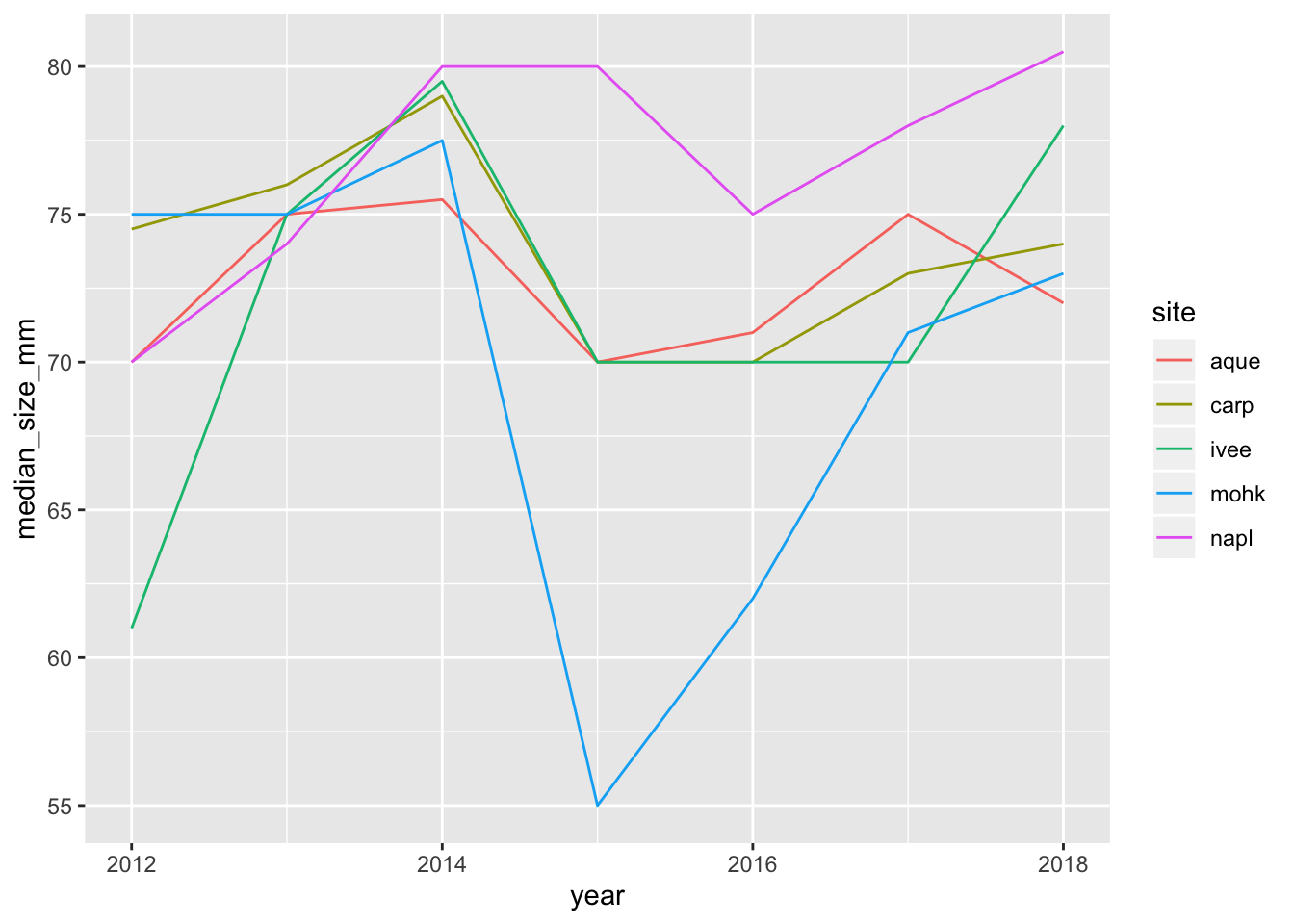
## Saving 7 x 5 in image## another option:
ggplot(siteyear_summary, aes(x = year, y = median_size_mm)) +
geom_col() +
facet_wrap(~site)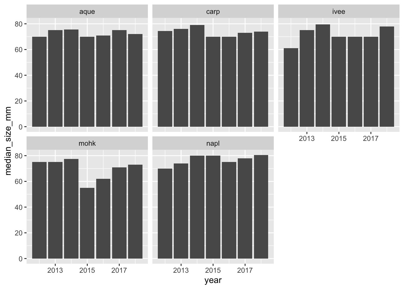
## Saving 7 x 5 in image7.8.1 Knit, push, & show differences on GitHub
So cool.
7.8.2 dplyr::count()
Now that we’ve spent time with group_by %>% summarize, there is a shortcut if you only want to summarize by count. This is with a function called count(), and it will group_by your selected variable, count, and then also ungroup. It looks like this:
lobsters %>%
  count(site, year)

## This is the same as:
lobsters %>%
  group_by(site, year) %>%
  summarize(n = n()) %>%
  ungroup()
Switching gears…
7.9 mutate()
There are a lot of times where you don’t want to summarize your data, but you do want to operate beyond the original data. This is often done by adding a column. We do this with the mutate() function from dplyr. Let’s try this with our original lobsters data. The sizes are in millimeters but let’s say it was important for them to be in meters. We can add a column with this calculation:
## # A tibble: 6 x 7
##    year month date    site  transect replicate size_mm
##   <dbl> <dbl> <chr>   <chr>    <dbl> <chr>       <dbl>
## 1  2012     8 8/20/12 ivee         3 A              70
## 2  2012     8 8/20/12 ivee         3 B              60
## 3  2012     8 8/20/12 ivee         3 B              65
## 4  2012     8 8/20/12 ivee         3 B              70
## 5  2012     8 8/20/12 ivee         3 B              85
## 6 2012 8 8/20/12 ivee 3 C 60## # A tibble: 6,366 x 8
## year month date site transect replicate size_mm size_m
## <dbl> <dbl> <chr> <chr> <dbl> <chr> <dbl> <dbl>
## 1 2012 8 8/20/12 ivee 3 A 70 0.07
## 2 2012 8 8/20/12 ivee 3 B 60 0.06
## 3 2012 8 8/20/12 ivee 3 B 65 0.065
## 4 2012 8 8/20/12 ivee 3 B 70 0.07
## 5 2012 8 8/20/12 ivee 3 B 85 0.085
## 6 2012 8 8/20/12 ivee 3 C 60 0.06
## 7 2012 8 8/20/12 ivee 3 C 65 0.065
## 8 2012 8 8/20/12 ivee 3 C 67 0.067
## 9 2012 8 8/20/12 ivee 3 D 70 0.07
## 10 2012 8 8/20/12 ivee 4 B 85 0.085
## # … with 6,356 more rowsIf we want to add a column that has the same value repeated, we can pass it just one value, either a number or a character string (in quotes). And let’s save this as a variable called lobsters_detailed
7.10 select()
We will end with one final function, select. This is how to choose, retain, and move your data by columns:
Let’s say that we want to present this data finally with only columns for date, site, and size in meters. We would do this:
## # A tibble: 6,366 x 3
##    date    site  size_m
##    <chr>   <chr>  <dbl>
##  1 8/20/12 ivee   0.07
##  2 8/20/12 ivee   0.06
##  3 8/20/12 ivee   0.065
##  4 8/20/12 ivee   0.07
##  5 8/20/12 ivee   0.085
##  6 8/20/12 ivee   0.06
##  7 8/20/12 ivee   0.065
##  8 8/20/12 ivee   0.067
##  9 8/20/12 ivee   0.07
## 10 8/20/12 ivee   0.085
## # … with 6,356 more rows
One last time, let’s knit, save, commit, and push to GitHub.
7.11 Deep thoughts
Highly recommended read: Broman & Woo: Data organization in spreadsheets. Practical tips to make spreadsheets less error-prone, easier for computers to process, easier to share
Great opening line: “Spreadsheets, for all of their mundane rectangularness, have been the subject of angst and controversy for decades.”
7.12 Efficiency Tips
arrow keys with shift, option, command