Chapter 10 Synthesis

10.1 Summary

In this session, we’ll pull together the skills that we’ve learned so far. We’ll create a new GitHub repo and R project, wrangle and visualize data from spreadsheets in R Markdown, communicate between RStudio (locally) and GitHub (remotely) to keep our updates safe, then share our outputs in a nicely formatted GitHub ReadMe. And we’ll learn a few new things along the way!

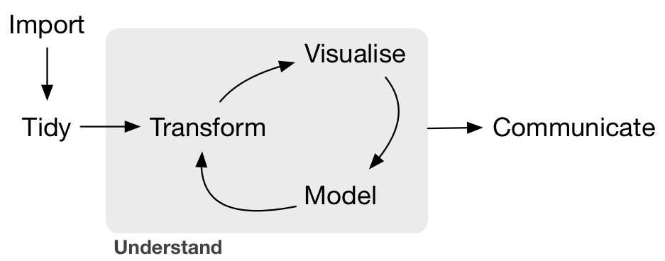
Grolemund & Wickham R4DS Illustration

10.2 Objectives

Create a new repo on GitHub
Start a new R project, connected to the repo
Create a new R Markdown document
Attach necessary packages (googlesheets4, tidyverse, here)
Use here::here() for simpler (and safer) file paths
Read in data from a Google sheet with the googlesheets4 package in R
Basic data wrangling (dplyr, tidyr, etc.)
Data visualization (ggplot2)
Publish with a useful ReadMe to share

10.3 Resources

The here package
googlesheets4 information
Project oriented workflows by Jenny Bryan

10.4 Lesson

10.4.1 Set-up:

Log in to your GitHub account and create a new repository called sea-creature-synthesis
Clone the repo to create a version controlled project (remember, copy & paste the URL from the GitHub Clone / Download)
In the local project folder, create a subfolder called ‘data’
Copy and paste the fish_counts_curated.csv and lobster_counts.csv into the ‘data’ subfolder
Create a new R Markdown document within your sea-creature-synthesis project
Knit your .Rmd to html, saving as sb_sea_creatures.Rmd

10.4.2 Attach packages and read in the data

Attach (load) packages with library():

library(tidyverse)
library(googlesheets4)
library(here)  
library(janitor)

Now we’ll read in our files with readr::read_csv(), but our files aren’t in our project root. They’re in the data subfolder.

Use here::here() to direct R where to look for files, if they’re not in the project root. Not sure where that is? Type here() in the Console, and it will tell you!

here::here()

"/returns/your/project/root/"

Go ahead, find your project root!

Then use here::here() again to easily locate a file somewhere outside of the exact project root. In our case, the files we want to read in are in the data subfolder - so we have to tell R how to get there from the root:

# Read in CSV files
fish_counts <- readr::read_csv(here::here("data", "fish_counts_curated.csv"))
lobster_counts <- readr::read_csv(here::here("data", "lobster_counts.csv"))

Check out the two data frames (fish_counts and lobster_counts).

The fish_counts data frame is in pretty good shape. But the lobster_counts df could use some love, because there are “-99999” entries indicating NA values, and the column names would be difficult to write code with.

When reading in the lobster data, let’s:

convert every “-99999” to an NA
get the column names into lower snake case using janitor::clean_names()

lobster_counts <- read_csv(here::here("curation", "lobster_counts.csv"),
                           na = "-99999") %>% 
                  clean_names()

Look at it again to check (always look at your data) - now both data frames seem pretty coder-friendly to work with.

10.4.3 Data wrangling

join?
filter?
unite/separate
Read in lobster data
Join with another existing data frame (or 2?)
Pivoting
Transforming / subsetting
Grouping & summarizing (for means, sd, count)
Make a table
Make a graph

Possible new things: complete()

R for Excel Users