Chapter 8 Tidying
TODO: janitor: adorn and kable
8.1 Summary
In previous sessions, we learned to read in data, do some wrangling, and create a graph and table. Here, we’ll continue by reshaping data frames (converting from long-to-wide, or wide-to-long format), separating and uniting variable (column) contents, converting between explicit and implicit missing (NA) values, and cleaning up our column names with the janitor package.
8.2 Objectives
- Reshape data frames with
tidyr::pivot_wider()andtidyr::pivot_longer() - Convert column names with
janitor::clean_names() - Combine or separate information from columns with
tidyr::unite()andtidyr::separate() - Make implicit missings explicit with
tidyr::complete() - Make explicit missings implicit with
tidyr::drop_na() - Use our new skills as part of a bigger wrangling sequence
- Make a customized table (TODO: or introduce Kable if not time in pivot tables chapter)
8.3 Resources
– Ch. 12 Tidy Data, in R for Data Science by Grolemund & Wickham
- tidyr documentation from tidyverse.org
- janitor repo / information from Sam Firke
8.4 Lesson
8.4.1 Lesson Prep
8.4.1.1 Create a new R Markdown and attach packages
Within your day 2 R Project, create a new .Rmd. Attach the tidyverse, janitor and readxl packages with library(package_name). Knit and save your new .Rmd within the project folder.
8.4.1.2 Read in data
Use readxl::read_excel() to import the “invert_counts_curated.xlsx” data:
Be sure to explore the imported data a bit:
View()names()summary()
8.4.2 Reshaping with tidyr::pivot_longer() and tidyr::pivot_wider()
8.4.2.1 Wide-to-longer format with tidyr::pivot_longer()
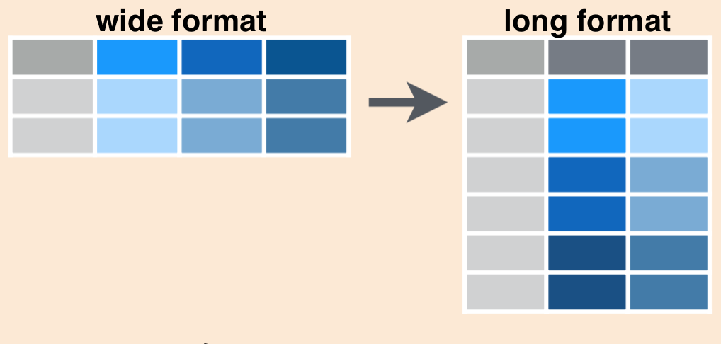
In tidy format, each variable is contained within a single column. If we look at inverts_df, we can see that the year variable is actually split over 3 columns, so we’d say this is currently in wide format.
There may be times when you want to have data in wide format, but often with code it is more efficient to convert to long format by gathering together observations for a variable that is currently split into multiple columns.
Schematically, converting from wide to long format looks like this:
Generally, the code to gather wide columns together using tidyr::pivot_longer() looks like this:
TODO: Add pivot_longer() schematic
We’ll use tidyr::pivot_longer() to gather data from all years in inverts_df into two columns: one called year, which contains the year (as a number), and another called sp_count that contains the number of each species observed. The new data frame will be stored as inverts_long:
inverts_long <- tidyr::pivot_longer(data = inverts_df,
                                    cols = '2016':'2018',
                                    names_to = "year",
                                    values_to = "sp_count")
The outcome is the new long-format inverts_long data frame:
## # A tibble: 165 x 5
##    month site  common_name              year  sp_count
##    <chr> <chr> <chr>                    <chr>    <dbl>
##  1 7     abur  california cone snail    2016       451
##  2 7     abur  california cone snail    2017        28
##  3 7     abur  california cone snail    2018       762
##  4 7     abur  california spiny lobster 2016        17
##  5 7     abur  california spiny lobster 2017        17
##  6 7     abur  california spiny lobster 2018        16
##  7 7     abur  orange cup coral         2016        24
##  8 7     abur  orange cup coral         2017        24
##  9 7     abur  orange cup coral         2018        24
## 10 7     abur  purple urchin            2016        48
## # … with 155 more rows
Hooray, long format!
One thing that isn’t obvious at first (but would become obvious if you continued working with this data) is that since those year numbers were initially column names (characters), when they are stacked into the year column, their class wasn’t auto-updated to numeric.
Explore the class of year in inverts_long:
## [1] "character"We’ll use dplyr::mutate() in a different way here: to create a new column (that’s how we’ve used mutate() previously) that has the same name of an existing column, in order to update and overwrite the existing column.
In this case, we’ll mutate() to add a column called year, which contains an as.numeric() version of the existing year variable:
Checking the class again, we see that year has been updated to a numeric variable:
## [1] "numeric"8.4.2.2 Long-to-wider format with tidyr::pivot_wider()
In the previous example, we had information spread over multiple columns that we wanted to gather. Sometimes, we’ll have data that we want to spread over multiple columns.
For example, imagine that starting from inverts_long we want each species in the common_name column to exist as its own column. In that case, we would be converting from a longer to a wider format, and will use tidyr::pivot_wider() as follows:
TODO: Add pivot_wider() schematic
Specifically for our data, we write code to spread the common_name column as follows:
inverts_wide <- inverts_long %>%
  tidyr::pivot_wider(names_from = common_name,
values_from = sp_count)## # A tibble: 33 x 8
## month site year `california con… `california spi… `orange cup cor…
## <chr> <chr> <dbl> <dbl> <dbl> <dbl>
## 1 7 abur 2016 451 17 24
## 2 7 abur 2017 28 17 24
## 3 7 abur 2018 762 16 24
## 4 7 ahnd 2016 27 16 24
## 5 7 ahnd 2017 24 16 24
## 6 7 ahnd 2018 24 16 24
## 7 7 aque 2016 4971 48 1526
## 8 7 aque 2017 1752 48 1623
## 9 7 aque 2018 2616 48 1859
## 10 7 bull 2016 1735 24 36
## # … with 23 more rows, and 2 more variables: `purple urchin` <dbl>, `rock
## # scallop` <dbl>We can see that now each species has its own column (wider format). But also notice that those column headers (since they have spaces) might not be in the most coder-friendly format…
8.4.2.3 Meet the janitor package
The janitor package by Sam Firke is a brilliant collection of functions for some quick data cleaning. We recommend that you explore the different functions it contains. Like:
janitor::clean_names(): update column headers to a case of your choosingjanitor::get_dupes(): see all rows that are duplicates within variables you choosejanitor::remove_empty(): remove empty rows and/or columnsjanitor::andorn_*(): jazz up frequency tables of counts (we’ll return to this for a table example in TODO: Session 8)- …and more!
Here, we’ll use janitor::clean_names() to convert all of our column headers to a more convenient case - the default is lower_snake_case, which means all spaces and symbols are replaced with an underscore (or a word describing the symbol), all characters are lowercase, and a few other nice adjustments.
For example, janitor::clean_names() would update these nightmare column names into much nicer forms:
My...RECENT-income!becomesmy_recent_incomeSAMPLE2.!test1becomessample2_test1ThisIsTheNamebecomesthis_is_the_name2015becomesx2015
If we wanted to then use these columns (which we probably would, since we created them), we could clean the names to get them into more coder-friendly lower_snake_case with janitor::clean_names():
## [1] "month"                    "site"
## [3] "year"                     "california_cone_snail"
## [5] "california_spiny_lobster" "orange_cup_coral"
## [7] "purple_urchin"            "rock_scallop"
And there are other options for the case, like:
- “snake” produces snake_case
- “lower_camel” or “small_camel” produces lowerCamel
- “upper_camel” or “big_camel” produces UpperCamel
- “screaming_snake” or “all_caps” produces ALL_CAPS
- “lower_upper” produces lowerUPPER
- “upper_lower” produces UPPERlower
8.4.3 Combine or separate information in columns with tidyr::unite() and tidyr::separate()
Sometimes we’ll want to separate contents of a single column into multiple columns, or combine entries from different columns into a single column.
For example, the following data frame has genus and species in separate columns:| id | genus | species | common_name |
|---|---|---|---|
| 1 | Scorpaena | guttata | sculpin |
| 2 | Sebastes | miniatus | vermillion |
| id | scientific_name | common_name |
|---|---|---|
| 1 | Scorpaena guttata | sculpin |
| 2 | Sebastes miniatus | vermillion |
Or we may want to do the reverse (separate information from a single column into multiple columns). Here, we’ll learn tidyr::unite() and tidyr::separate() to help us do both.
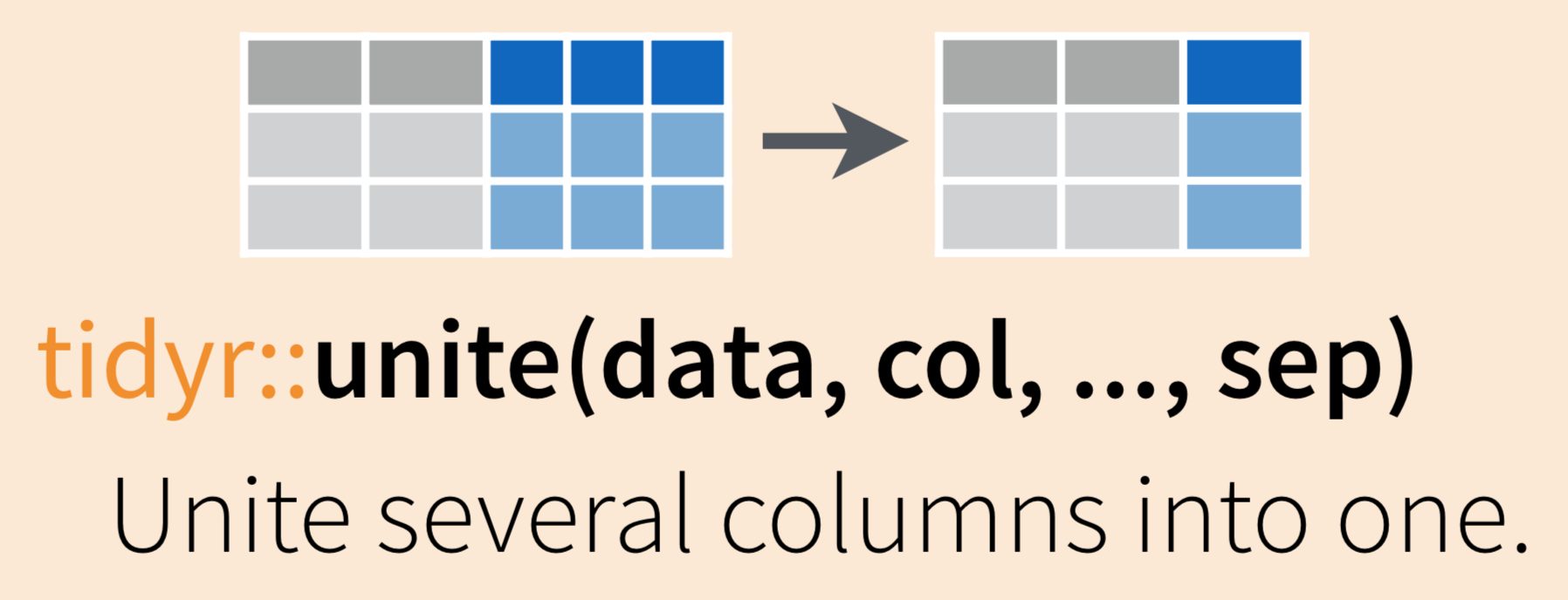
8.4.3.1 tidyr::unite() to merge information from separate columns
Use tidyr::unite() to combine (paste) information from multiple columns into a single column (as for the scientific name example above)
To demonstrate uniting information from separate columns, we’ll make a single column that has the combined information from site abbreviation and year in inverts_wide.
We need to give tidyr::unite() several arguments:
- data: the data frame containing columns we want to combine (or pipe into the function from the data frame)
- col: the name of the new “united” column
- the columns you are uniting
- sep: the symbol, value or character to put between the united information from each column
inverts_unite <- inverts_wide %>%
  tidyr::unite(col = "site_year", # What to name the new united column
               c(site, year), # The columns we'll unite (site, year)
               sep = "_") # How to separate the things we're uniting
## # A tibble: 6 x 7
## month site_year california_cone… california_spin… orange_cup_coral
## <chr> <chr> <dbl> <dbl> <dbl>
## 1 7 abur_2016 451 17 24
## 2 7 abur_2017 28 17 24
## 3 7 abur_2018 762 16 24
## 4 7 ahnd_2016 27 16 24
## 5 7 ahnd_2017 24 16 24
## 6 7 ahnd_2018 24 16 24
## # … with 2 more variables: purple_urchin <dbl>, rock_scallop <dbl>Try updating the separator from "_" to “hello!” to see what the outcome column contains.
tidyr::unite() can also combine information from more than two columns. For example, to combine the site, common_name and year columns from inverts_long, we could use:
# Uniting more than 2 columns:

inverts_triple_unite <- inverts_long %>%
  tidyr::unite(col = "year_site_name",
               c(year, site, common_name),
sep = "-")## # A tibble: 6 x 3
## month year_site_name sp_count
## <chr> <chr> <dbl>
## 1 7 2016-abur-california cone snail 451
## 2 7 2017-abur-california cone snail 28
## 3 7 2018-abur-california cone snail 762
## 4 7 2016-abur-california spiny lobster 17
## 5 7 2017-abur-california spiny lobster 17
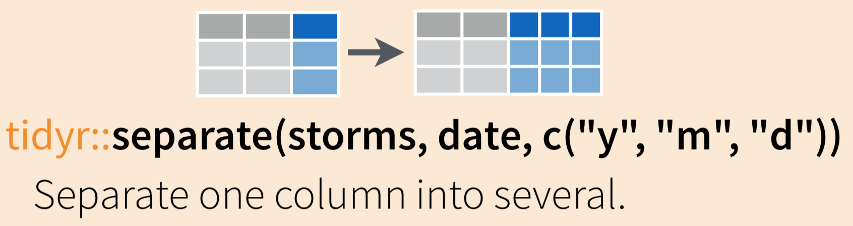
## 6 7 2018-abur-california spiny lobster 168.4.3.2 tidyr::separate() to separate information into multiple columns
While tidyr::unite() allows us to combine information from multiple columns, it’s more likely that you’ll start with a single column that you want to split up into pieces.
For example, I might want to split up a column containing the genus and species (Scorpaena guttata) into two separate columns (Scorpaena | guttata), so that I can count how many Scorpaena organisms exist in my dataset at the genus level.
Use tidyr::separate() to “separate a character column into multiple columns using a regular expression separator.”
Let’s start again with inverts_unite, where we have combined the site and year into a single column called site_year. If we want to separate those, we can use:
inverts_sep <- inverts_triple_unite %>%
  tidyr::separate(year_site_name, into = c("my_year", "my_site_name"))
## Warning: Expected 2 pieces. Additional pieces discarded in 165 rows [1, 2, 3, 4,
## 5, 6, 7, 8, 9, 10, 11, 12, 13, 14, 15, 16, 17, 18, 19, 20, ...].What is that warning Expected 2 pieces... telling us? If we take a look at the resulting data frame inverts_sep, we see that it only keeps the first two pieces, and gets rid of the third (name). Which is a bit concerning, because we rarely want to just throw away information in a data frame.
## # A tibble: 6 x 4
##   month my_year my_site_name sp_count
##   <chr> <chr>   <chr>           <dbl>
## 1 7     2016    abur              451
## 2 7     2017    abur               28
## 3 7     2018    abur              762
## 4 7     2016    abur               17
## 5 7     2017    abur               17
## 6 7     2018    abur               16
That’s problematic. How can we make sure we’re keeping as many different elements as exist in the united column?
We have a couple of options:
- Create the number of columns that are needed to retain as many elements as exist (in this case, 3, but we only created two new columns in the example above)
inverts_sep3 <- inverts_triple_unite %>%
  tidyr::separate(year_site_name, into = c("the_year", "the_site", "the_name"))
## Warning: Expected 3 pieces. Additional pieces discarded in 165 rows [1, 2, 3, 4,
## 5, 6, 7, 8, 9, 10, 11, 12, 13, 14, 15, 16, 17, 18, 19, 20, ...].Another warning. What is that about? Let’s take a look at the resulting data frame and think about what’s missing (what are the “pieces discarded”?):
## # A tibble: 6 x 5
##   month the_year the_site the_name   sp_count
##   <chr> <chr>    <chr>    <chr>         <dbl>
## 1 7     2016     abur     california      451
## 2 7     2017     abur     california       28
## 3 7     2018     abur     california      762
## 4 7     2016     abur     california       17
## 5 7     2017     abur     california       17
## 6 7     2018     abur     california       16
Aha! Only the first word of the common name was retained, and anything else was trashed. We want to keep everything after the second dash in the new the_name column.
That’s because the default is extra = "warn", which means that if you have more pieces than columns you’re separating into, it will populate the columns that have been allotted (in our case, just 3) then drop any additional information, giving you a warning that pieces have been dropped.
To keep the extra pieces that have been dropped, add the extra = "merge" argument within tidyr::separate() to override:
inverts_sep_all <- inverts_triple_unite %>%
  separate(year_site_name,
           into = c("sample_year", "location", "sp_name"),
           extra = "merge")
No warning there about things being discarded. Explore inverts_sep_all:
## # A tibble: 165 x 5
##    month sample_year location sp_name                  sp_count
##    <chr> <chr>       <chr>    <chr>                       <dbl>
##  1 7     2016        abur     california cone snail         451
##  2 7     2017        abur     california cone snail          28
##  3 7     2018        abur     california cone snail         762
##  4 7     2016        abur     california spiny lobster       17
##  5 7     2017        abur     california spiny lobster       17
##  6 7     2018        abur     california spiny lobster       16
##  7 7     2016        abur     orange cup coral               24
##  8 7     2017        abur     orange cup coral               24
##  9 7     2018        abur     orange cup coral               24
## 10 7     2016        abur     purple urchin                  48
## # … with 155 more rows
We see that the resulting data frame has split year_site_name into three separate columns, sample_year, location, and sp_name, but now everything after the second break (“-”) remains together in sp_name instead of dropping pieces following the third word.
8.4.4 Convert between explicit and implicit missings (NAs)
An explicit missing is when every possible outcome actually appears in a data frame as a row, even if a variable of interest for that row is missing (NA).
Conversely, an implicit missing is when an observation (row) does not appear in the data frame because a variable of interest contains an NA missing value.
Consider the following data:
| day | animal | food_choice |
|---|---|---|
| Monday | eagle | fish |
| Monday | mountain lion | squirrel |
| Monday | toad | NA |
| Tuesday | eagle | fish |
| Tuesday | mountain lion | deer |
| Tuesday | toad | flies |
Notice that the row for toad still appears in the dataset for Tuesday, despite having a missing food choice for that day. This is an explicit missing because the row still appears in the data frame.
If that row was removed, the resulting dataset would look like this:
| day | animal | food_choice |
|---|---|---|
| Monday | eagle | fish |
| Monday | mountain lion | squirrel |
| Tuesday | eagle | fish |
| Tuesday | mountain lion | deer |
| Tuesday | toad | flies |
…and if your reaction is “But then how do I know there’s a toad from MONDAY?”, then you can see how it can be a bit risky to have implicit missings instead of explicit missings.
Whichever we choose, we can convert between the two forms using tidyr::drop_na() or tidyr::complete():
tidyr::drop_na(): removes observations (rows) that containNAfor variable(s) of interesttidyr::complete(): turns implicit missing values into explicit missing values by completing a data frame with missing combinations of data
We’ll use both here, starting with the inverts_long data frame we created above.
Looking through inverts_long, we’ll see that there are NA observations for every species at site bull in 2018 - but those NA counts do show up. First, we’ll use tidyr::drop_na() to make those missings implicit (invisible) instead:
See that now, the rows that contained an NA in the sp_count column from inverts_long have been removed.
WAIT, I want them back! We can ask R to create explicit missings (by identifying which combinations of groups currently don’t appear in the data frame) using tidyr::complete():
Now you’ll see inverts_explicit_NA has those 5 “missing” observations shown in the data frame.
8.4.5 Activities
TODO
8.4.6 Fun facts / insights
TODO