Chapter 3 R & RStudio, RMarkdown
3.1 Summary
We’ll learn RMarkdown, which helps you tell a story with your data analysis because you can write text alongside the code. We are actually learning two languages at once: R and Markdown.
3.1.1 Objectives
In this lesson we will:
- get oriented to the RStudio interface
- work with R in the console
- be introduced to built-in R functions
- learn to use the help pages
- explore RMarkdown
3.1.2 Resources
- R for Excel Users by Gordon Shotwell (blog)
3.2 Why learn R with RStudio
You are all here today to learn how to code. Coding made me a better scientist because I was able to think more clearly about analyses, and become more efficient in doing so. Data scientists are creating tools that make coding more intuitive for new coders like us, and there is a wealth of awesome instruction and resources available to learn more and get help.
Here is an analogy to start us off. Think of yourself as a pilot, and R is your airplane. You can use R to go places! With practice you’ll gain skills and confidence; you can fly further distances and get through tricky situations. You will become an awesome pilot and can fly your plane anywhere.
And if R were an airplane, RStudio is the airport. RStudio provides support! Runways, communication, community, and other services that makes your life as a pilot much easier. So it’s not only the infrastructure (the user interface or IDE), although it is a great way to learn and interact with your variables, files, and interact directly with GitHub. It’s also a data science philosophy, R packages, community, and more. So although you can fly your plane without an airport and we could learn R without RStudio, that’s not what we’re going to do.
We are learning R together with RStudio and its many supporting features.
3.3 RStudio Orientation
Open RStudio for the first time.
Launch RStudio/R.

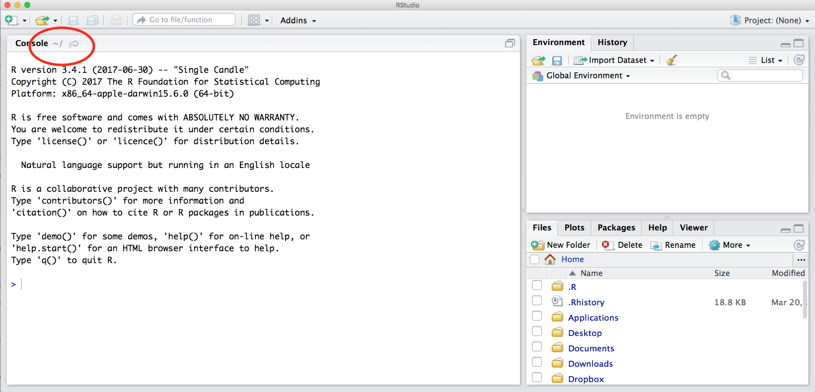
Notice the default panes:
- Console (entire left)
- Environment/History (tabbed in upper right)
- Files/Plots/Packages/Help (tabbed in lower right)
FYI: you can change the default location of the panes, among many other things: Customizing RStudio.
An important first question: where are we?
If you’ve have opened RStudio for the first time, you’ll be in your Home directory. This is noted by the ~/ at the top of the console. You can see too that the Files pane in the lower right shows what is in the Home directory where you are. You can navigate around within that Files pane and explore, but note that you won’t change where you are: even as you click through you’ll still be Home: ~/.
3.3.1 R Console
OK let’s go into the Console, where we interact with the live R process.
We can do math:
But like Excel, the power comes not from doing small operations by hand (like 8*22.3), it’s by being able to operate on whole suites of numbers and datasets. In Excel, data are stored in the spreadsheet. In R, they are stored in objects, which are often vectors or dataframes. They are rectangular.
3.3.2 Viewing data in R
Let’s have a look at some data in R. Unlike Excel, R comes out-of-the-box with several built-in data sets that we can look at and work with.
One of these datasets is called cars. If I write this in the Console, it will print the data in the console.
This returns data. To me this is not super interesting data, but I can appreciate that there are different variables listed as column headers and then numeric values for each type of row observation. (Unfortunately I don’t know if these are different cars or trials or conditions but we won’t focus on that for now).
I can also use RStudio’s Viewer to see this in a more familiar-looking format. Let’s type this — and make sure it’s a capital V and open and closed parentheses:
This opens the fourth pane of the RStudio IDE; when you work in R you will have all four panes open so this will become a very comforting setup for you.
Aside The basic R data structure is a vector. You can think of a vector like a column in an Excel spreadsheet with the limitation that all the data in that vector must be of the same type. If it is a character vector, every element must be a character; if it is a logical vector, every element must be TRUE or FALSE; if it’s numeric you can trust that every element is a number. There’s no such constraint in Excel: you might have a column which has a bunch of numbers, but then some explanatory test intermingled with the numbers. This isn’t allowed in R. - Gordon Shotwell
In the Viewer I can do things like filter or sort. This does not do anything to the actual data, it just changes how you are viewing the data. So even as I explore it, I am not editing or manipulating the data.
3.3.3 R functions, help pages
Like Excel, some of the biggest power in R is that there are built-in functions that you can use in your analyses (and, as we’ll see, R users can easily create and share functions, and it is this open source developer and contributor community that makes R so awesome).
R has a mind-blowing collection of built-in functions that are used with the same syntax: function name with parentheses around what the function needs to do what it is supposed to do. function_name(argument1 = value1, argument2 = value2, ...). When you see this syntax, we say we are “calling the function”.
Let’s try using seq() which makes regular sequences of numbers and, while we’re at it, demo more helpful features of RStudio.
Type se and hit TAB. A pop up shows you possible completions. Specify seq() by typing more to disambiguate or using the up/down arrows to select. Notice the floating tool-tip-type help that pops up, reminding you of a function’s arguments. If you want even more help, press F1 as directed to get the full documentation in the help tab of the lower right pane.
Type the arguments 1, 10 and hit return.
## [1] 1 2 3 4 5 6 7 8 9 10We could probably infer that the seq() function makes a sequence, but let’s learn for sure. Type (and you can autocomplete) and let’s explore the help page:
When I press enter/return, it will open up a help page in the bottom right pane. Help pages vary in detail I find some easier to digest than others. But they all have the same structure, which is helpful to know. The help page tells the name of the package in the top left, and broken down into sections:
- Description: An extended description of what the function does.
- Usage: The arguments of the function and their default values.
- Arguments: An explanation of the data each argument is expecting.
- Details: Any important details to be aware of.
- Value: The data the function returns.
- See Also: Any related functions you might find useful.
- Examples: Some examples for how to use the function.
When I look at a help page, I start with the description, which might be too in-the-weeds for the level of understanding I need at the offset. For the sum page, it is pretty straight-forward and lets me know that yup, this is the function I want.
I next look at the usage and arguments, which give me a more concrete view into what the function does. This syntax looks a bit cryptic but what it means is that you use it by writing sum, and then passing whatever you want to it in terms of data: that is what the “…” means. And the “na.rm=FALSE” means that by default, it will not remove NAs (I read this as: “remove NAs? FALSE!”)
Then, I usually scroll down to the bottom to the examples. This is where I can actually see how the function is used, and I can also paste those examples into the Console to see their output. Let’s try it:
## [1] 1 2 3 4 5 6 7 8 9 10## [1] 1 3 5 7 9The above also demonstrates something about how R resolves function arguments. You can always specify in name = value form. But if you do not, R attempts to resolve by position. So above, it is assumed that we want a sequence from = 1 that goes to = 10. Since we didn’t specify step size, the default value of by in the function definition is used, which ends up being 1 in this case. For functions I call often, I might use this resolve by position for the first
argument or maybe the first two. After that, I always use name = value.
The examples from the help pages can be copy-pasted into the console for you to understand what’s going on. Remember we were talking about expecting there to be a function for something you want to do? Let’s try it.
3.3.4 Activity
Exercise: Talk to your neighbor(s) and look up the help file for a function that you know or expect to exist. Here are some ideas:
?getwd(),?plot(),min(),max(),?mean(),?log()).
Let’s try another. In Excel, there is a “SUM” function to calculate a total. Let’s expect that there is the same in R. I will type this into the Console:
R is case-sensitive. So “sum” is a completely different thing to “Sum” or “SUM”. And this is true for the names of functions, data sets, variable names, and data itself (“blue” vs “Blue”).
Awesome. Let’s try this on our cars data
Alright. What is this number? It is the sum of ALL of the data in the cars dataset. Maybe in some analysis this would be a useful operation, but I would worry about the way your data is set up and your analyses if this is ever something you’d want to do. More likely, you’d want to take the sum of a specific column. In R, you can do that with the $ operator.
Let’s say we want to calculate the total distance:
There are many functions that are built into R, and we’ll learn more of them shortly.
Not all functions have (or require) arguments:
## [1] "Mon Feb 3 09:00:59 2020"3.3.5 Packages
So far we’ve been using a couple functions from base R, such as sum() and date(). But, one of the amazing things about R is that a vast user community is always creating new functions and packages that expand R’s capabilities. In R, the fundamental unit of shareable code is the package. A package bundles together code, data, documentation, and tests, and is easy to share with others. They increase the power of R by improving existing base R functionalities, or by adding new ones.
The traditional place to download packages is from CRAN, the Comprehensive R Archive Network, which is where you downloaded R. You can also install packages from GitHub, which we’ll do tomorrow.
You don’t need to go to CRAN’s website to install packages, this can be accomplished within R using the command install.packages("package-name-in-quotes"). Let’s install a small, fun package praise. You need to use quotes around the package name.
Do this in the Console instead of in your RMarkdown file because we don’t want this to load every time:
Now we’ve installed the package, but we need to tell R that we are going to use the functions within the praise package. We do this by using the function library().
In my mind, this is analogous to needing to wire your house for electricity: this is something you do once; this is install.packages. But then you need to turn on the lights each time you need them (R Session).
Now that we’ve loaded the praise package, we can use the single function in the package, praise(), which returns a randomized praise to make you feel better.
## [1] "You are solid!"3.3.6 Assigning objects with <-
This might be a really important value that we want to have on hand. We can save this as its own object.
This is a big difference with Excel, where you usually identify data by its location on the grid, like $A1:D$20. (You can do this with Excel by naming ranges of cells, but many people don’t do this.)
Data can be a variety of formats, like numeric and text.
We do this by writing the name along with the assignment operator <-
And we can execute it. In my head I hear “sum_dist gets 2149”.
Object names can be whatever you want, although they cannot start with a digit and cannot contain certain other characters such as a comma or a space. Different folks have different conventions; you will be wise to adopt a convention for demarcating words in names.
Notice that as I start typing sum_dist in the Console, there will be options to auto-fill. This is RStudio helping you out, which is great because we all are prone to typos. I actually have to ignore the help to try to force a typo:
OK this is an error, but I didn’t break R — error messages are your friends.
The first thing to do with an error message is read it. Yes it’s in angry red text and it’s unexpected — but most error messages are doing their best to help you solve the problem. And you’ll get more familiar with they way they tell you. By saying “object ‘sumdist’ not found” alerts me immediately to the fact that this thing I think exists R doesn’t think exists — so maybe it’s a typo or not loaded?
3.3.7 Error messages are your friends
As Jenny Bryan says:
Implicit contract with the computer / scripting language: Computer will do tedious computation for you. In return, you will be completely precise in your instructions. Typos matter. Case matters. Pay attention to how you type.
Remember that this is a language, not unsimilar to English! There are times you aren’t understood – it’s going to happen. There are different ways this can happen. Sometimes you’ll get an error. This is like someone saying ‘What?’ or ‘Pardon’? Error messages can also be more useful, like when they say ‘I didn’t understand what you said, I was expecting you to say blah’. That is a great type of error message. Error messages are your friend. Google them (copy-and-paste!) to figure out what they mean.
And also know that there are errors that can creep in more subtly, when you are giving information that is understood, but not in the way you meant. Like if I am telling a story about suspenders that my British friend hears but silently interprets in a very different way (true story). This can leave me thinking I’ve gotten something across that the listener (or R) might silently interpreted very differently. And as I continue telling my story you get more and more confused… Clear communication is critical when you code: write clean, well documented code and check your work as you go to minimize these circumstances!
3.3.8 Logical operators and expressions
A moment about logical operators and expressions. We can ask questions about the objects we made. This is not assigning a new value to our sum_dist object.
==means ‘is equal to’!=means ‘is not equal to’<means ` is less than’>means ` is greater than’<=means ` is less than or equal to’>=means ` is greater than or equal to’
## [1] FALSE## [1] TRUE## [1] TRUEShortcuts You will make lots of assignments and the operator
<-is a pain to type. Don’t be lazy and use=, although it would work, because it will just sow confusion later. Instead, utilize RStudio’s keyboard shortcut: Alt + - (the minus sign). Notice that RStudio automagically surrounds<-with spaces, which demonstrates a useful code formatting practice. Code is miserable to read on a good day. Give your eyes a break and use spaces. RStudio offers many handy keyboard shortcuts. Also, Alt+Shift+K brings up a keyboard shortcut reference card.
My most common shortcuts include command-Z (undo), and combinations of arrow keys in combination with shift/option/command (moving quickly up, down, sideways, with or without highlighting.
3.4 Clearing the environment
Now look at the objects in your environment (workspace) – in the upper right pane. The workspace is where user-defined objects accumulate.
For reproducibility, it is critical that you delete your objects and restart your R session frequently. You don’t want your whole analysis to only work in whatever way you’ve been working right now — you need it to work next week, after you upgrade your operating system, etc. Restarting your R session will help you identify and account for anything you need for your analysis.
We will keep coming back to this theme but let’s restart our R session together: Go to the top menus: Session > Restart R.
Don’t save the workspace!
So this is great, but if we were going to do any kind of real analysis, we need to be able to write it in a document rather than this command line prompt in the Console. Let’s do something much more interesting and really start feeling its power.
3.5 Intro to RMarkdown
An RMarkdown file is a special type of file for making reports — it allow us to weave markdown text with chunks of R code to be evaluated and output content like tables and plots.
This is really critical to reproducibility, and it also saves time. This document will recreate your figures for you in the same document where you are writing text. So no more doing analysis, saving a plot, pasting that plot into Word, redoing the analysis, re-saving, re-pasting, etc.
Let’s experience this a bit ourselves and then we’ll talk about it more.
3.5.1 Create an RMarkdown file
File -> New File -> RMarkdown… -> Document of output format HTML, OK.
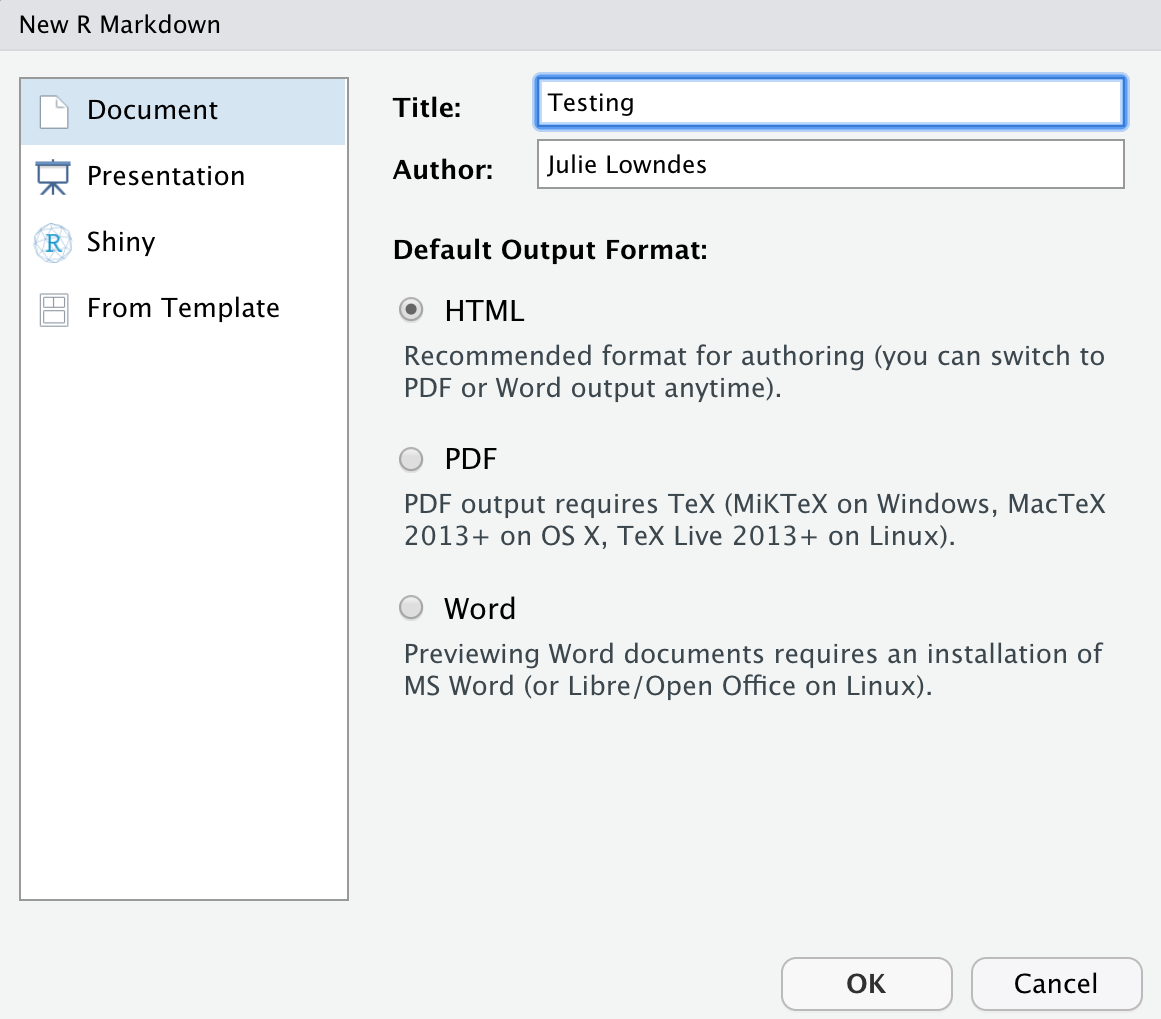
You can give it a Title like “Testing” (a name that’s totally ok to use as you’re trying something out). Then click OK.
OK, first off: by opening a file, we are seeing the 4th pane of the RStudio console, which is essentially a text editor. This lets us organize our files within RStudio instead of having a bunch of different windows open.
Let’s have a look at this file — it’s not blank; there is some initial text is already provided for you. Notice a few things about it:
- Title and Author are auto-filled, and the today’s date has been added
- There are white and grey sections. These are the 2 main languages that make up an RMarkdown file.
- Grey sections are R code
- White sections are Markdown text

3.5.2 Knit your RMarkdown file
Let’s go ahead and “Knit” by clicking the blue yarn at the top of the RMarkdown file. It’s going to ask us to save first, I’ll name mine “testing.Rmd”.
How cool is this, we’ve just made an html file, a webpage that we are viewing locally on our own computers. Knitting this RMarkdown document has rendered — we also say formatted — both the Markdown text (white) and the R code (grey), and the it also executed — we also say ran — the R code.
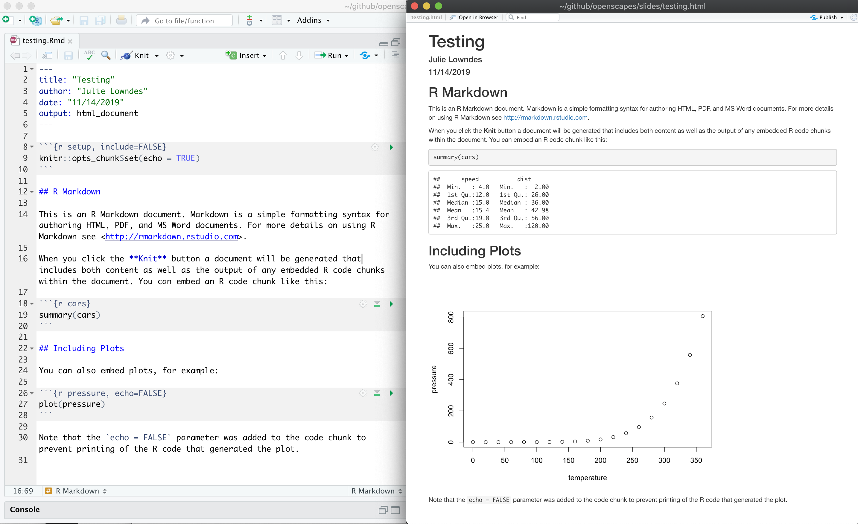
Let’s have a look at them side-by-side:
Let’s take a deeper look at these two files. So much of learning to code is looking for patterns.
3.5.3 R code chunks
Notice how the grey R code chunks are surrounded by 3 backticks and {r LABEL}. These are evaluated and return the output text in the case of summary(cars) and the output plot in the case of plot(pressure).
Notice how the code plot(pressure) is not shown in the HTML output because of the R code chunk option echo=FALSE.
We can create a new chunk in your RMarkdown first in one of these ways:
- click “Insert > R” at the top of the editor pane
- type by hand ```{r} ```
- if you haven’t deleted a chunk that came with the new file, edit that one
Now, let’s write some code in R. Earlier we calculated sum(cars$dist). Now let’s do the average. In R, this is the mean() function
Now, hitting return does not execute this command; remember, it’s a text file in the text editor, it’s not associated with the R engine. To execute it, we need to get what we typed in the the R chunk (the grey R code) down into the console. How do we do it? There are several ways (let’s do each of them):
- copy-paste this line into the console.
- select the line (or simply put the cursor there), and click ‘Run’. This is available from
- the bar above the file (green arrow)
- the menu bar: Code > Run Selected Line(s)
- keyboard shortcut: command-return
- click the green arrow at the right of the code chunk
And when we do this, we see the mean_dist object appear in he Environment pane.
Cool tip: doesn’t have to be only R, other languages supported.
3.5.4 Activity (3 min)
Calculate the maximum cars distance in your RMarkdown file by typing
max(cars$dist). Remember to write your R code within a code chunk (grey)!
Execute your commands by trying the three ways above. Then, knit your R Markdown file, which will also save the Rmd by default.
3.5.5 Markdown sections
The second language is Markdown. This is a formatting language for plain text, and there are only about 15 rules to know.
Notice the syntax for:
- headers get rendered at multiple levels:
#,## - bold:
**word**
There are some good cheatsheets to get you started, and here is one built into RStudio: Go to Help > Markdown Quick Reference
Learn more: http://rmarkdown.rstudio.com/
3.5.6 Activity
- In Markdown write some italic text, make a numbered list, and add a few subheaders. Use the Markdown Quick Reference (in the menu bar: Help > Markdown Quick Reference).
- Reknit your html file.
3.5.7 Restart R
To end our work from this session, save, knit, and then restart R (Go to the top menus: Session > Restart R.)
Notice that now with a clean workspace, if I knit my document instead of sending code to the Console, my objects (like mean_dist) don’t show up in my Environment. This is because R isn’t actually running this in this R session, it is actually spinning up a clean session to knit my document. This is important for reproducible analyses because I don’t want the success of this analysis to be dependent on some weird setting I have on my computer that will make Future Me or Future Us not able to run or understand these important analyses. Having RMarkdown be self-contained in this way helps you develop good habits for reproducibility.
3.5.8 What is RMarkdown? (1-minute video)
Let’s watch this to demonstrate all the amazing things you can now do:
3.6 Deep thoughts
Comments! Organization (spacing, subsections, vertical structure, indentation, etc.)! Well-named variables! Also, well-named operations so analyses (select(data, columnname)) instead of data[1:6,5] and excel equivalent. (Ex with strings) Not so brittle/sensitive to minor changes.